Random Forest is an easy and reliable algorithm that leverages multiple decision trees to predict an outcome. In this project, I used a Random Forest approach to predict the outcomes of NHL hockey games.

Data Collection

My goal in this project was to create a model that can be used in the present to predict the winner of a hockey game. To create this model, I decided to first use data from the previous (2022-2023) NHL season. I used the NHL’s official API to obtain my data.

After fetching the 2022-2023 schedule and the games, I was able to tabulate the scores of all ~1300 games played during the regular season. I also fetched the rosters for each team at the time (note, this model did not take into account that players could be traded mid season). Using the rosters, I tabulated the following data for each team:

• Goals per game
• Goals against per game
• Team combined plus minus
• Total penalty minutes
• Powerplay goals
• Shorthanded goals
• Shots per game
• Shots against per game
• Regulation wins

Data Analysis

Before I began the development of my model, I analyzed my data by using scatter plots to see how the stats above correlated to a team’s success.

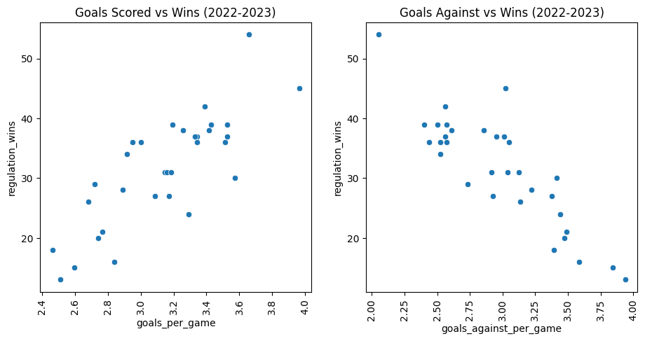
As expected, the two stats involving goals had a strong correlation to a team’s win rate:

Since the stats are heavily related, plus minus also had a similar relationship:

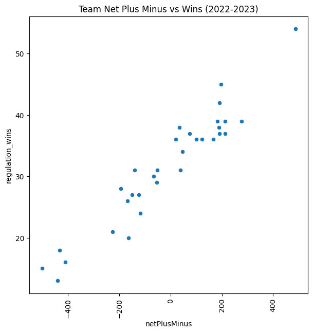
From the above data it is clear that teams that score more tend to win more, and teams that let in more goals win less. But what about teams that shoot more?

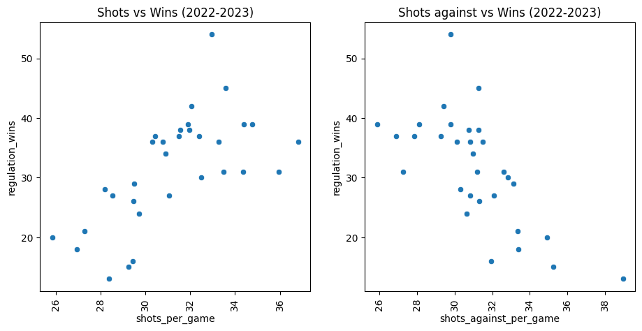
I was surprised to see the heavy effect of a team’s shots per game and shots allowed per game to a team’s success. In hockey, scoring chances from shots can range from a very probable goal (cross-crease one timer) to an almost guranteed save. On a game by game basis, there are many occasions where the team being outshot will come out with the victory. However, it is clear from this data that over the course of a season, the number of shots does matter to a team’s win rate. I graphed special teams data to check for a similar effect:

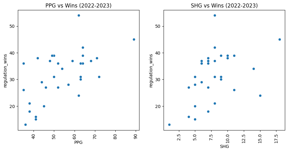
Apart from a few outliers, there is a small upward trend in scoring powerplay/shorthanded goals and winning. With penalty minutes, there is almost no relation at all:

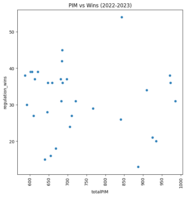
Based on that information, I should be able to generate a decision tree that compares two teams’ stats and picks a likely winner. Also, enforcers and tough hockey need to make a return to the NHL, as the data proved that penalty minutes don’t have much affect on a team’s season. The 2010-2011 Boston Bruins will forever be in my heart as the greatest team in NHL history. Special shoutout to Zdeno Chara, Shawn Thornton, Adam McQuaid, Andrew Ference, Johnny Boychuck, Nathan Horton, Tim Thomas and more.

Creating a decision tree

To create a decision tree, I went to each game in the season and fetched the stats for the opposing teams. For my independant “x” variables, I created a boolean variable for each stat. For example, if the home team had a higher goals per game than the away team, home_more_goals was set to True (I removed the plus minus stat for this step since goals for and goals against essentially add up to that stat). In this case, the dependant “y” variable was whether or not the home team won, which I had tabulated earlier.

Using sklearn’s DecisionTreeClassifer class, I was able to create a Decision Tree without having to manually split my data. I used the graphviz library to display a visual of the tree, and after playing around with the hyperparameters, I came up with this:

In this diagram, nodes with a darker blue represent outcomes where the home team is more likely to win and the darker orange represent outcomes where the away team is more likely to win. Nodes that are lighter in shade are less certain of one particular outcome. Samples represents the number of games used at each node, and values shows the split between the away team winning and the home team winning in those games. Gini is a score of a node’s impurity, and in this context, it represents the likelyhood of selecting two games from a sample that have the same homeWin outcome.

The decision tree maps out sequences of boolean outcomes where we can classify our known data to see if the home team won in that particular matchup. From the above, we can see that there were 113 games where the home team had a lower goals against rate, higher goals for rate, higher short handed goal rate, higher powerplay goal rate, and more total penalty minutes (see far right leaf). In those 113 games, the home team won 84 times, which makes sense, as almost every stat listed were in their favour.

Creating a random forest

A random forest is an ensemble of decision trees that take a random (with replacement) subset of the data. To get a final prediction of an outcome, we take the average of the predictions from all of the models. This is more accurate than using one decision tree, because the average of a large number of uncorrelated random errors is 0. Creating a random tree is quite simple using the sklearn RandomForestClassifier class.

After creating a random forest I plotted the feature importance of the model:

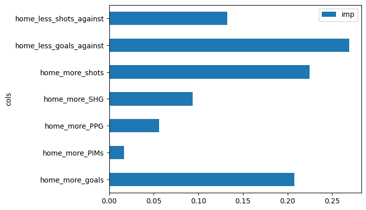
The most important factors for predicting games in my model were goals against average, shots per game, and goals per game. Special teams and penalty minutes had low importance in my model.

For the test set, I fetched the scores (approx. 800 games) up until today’s (02-14-2024) date in the current NHL season and fetched this season’s stats for each team (using the same functions as before). I used the predict method for the RandomForestClassifier class, which produced a ~800x1 matrix of boolean values homeWin. I then compared these predictions to the actual results of the games, which gave me my accuracy score.

Optimizing Hyperparameters

When creating a RandomForestClassifier object, you get to set the following parameters:

RandomForestClassifier(n_estimators=100, *, criterion='gini', max_depth=None, min_samples_split=2, min_samples_leaf=1, min_weight_fraction_leaf=0.0, max_features='sqrt', max_leaf_nodes=None, min_impurity_decrease=0.0, bootstrap=True, oob_score=False, n_jobs=None, random_state=None, verbose=0, warm_start=False, class_weight=None, ccp_alpha=0.0, max_samples=None, monotonic_cst=None)

These parameters give you control over attributes like complexity, performance, and ultimately the accuracy of the Random Forest classifier. In the previous step, I started with arbitrary values for some of the parameters and tweaked them manually to seemingly train the “best” model. The values I ended up with were:

n_estimators = 200 # Number of trees in the forest (higher is typically better but comes at cost of training time)
bootstrap = True # Each tree is built using a random subset (with replacement) of the data (instead of using the entire dataset)
max_samples = 500 # Number of samples to draw from the dataset to train each tree
max_depth = 5 # Maximum depth of each tree. Too high can result in overfitting
min_samples_leaf = 60 # Minimum number of samples at each node in the tree

The model with the above parameter produces an accuracy of 63%, which is pretty good.

While intuition and brute force could be used to find the best combination of parameters, there are quicker and automated ways to do so. I used the RandomizedSearchedCV class from sklearn to test different hyperparameter values. My parameter space looked like this:

params = {
    "n_estimators": [100, 200, 300, 400, 500],
    "max_samples": [100, 200, 300, 400, 500],
    "max_depth": [5, 10, 15, 20, 25],
    "min_samples_leaf": [10, 20, 30, 40, 50]
}   

The RandomizedSearchCV will choose N combinations from this space, and return the combination that yielded the best result. I chose N = 10 to save time:

clf = RandomizedSearchCV(rf, params, n_iter=10, cv=5, n_jobs=-1)

The output was a combination of hyperparameters that was quite different from my original values!

{'n_estimators': 500,
 'min_samples_leaf': 10,
 'max_samples': 400,
 'max_depth': 10}

These changes to the parameters boosted my model’s accuracy from 63% to 64%, which, although is a small change, shows the potential returns of using strategies like hyperparameter tuning.

Conclusion

The final accuracy of my model in predicting NHL games was 0.6422018348623854 or 64%. While this may seem low, one should note that the ‘favourites’ in sportsbooks for hockey have a win rate of approximately 60%. This means that the team with the higher odds of winning (set by the sportsbook) win 60% of the time.

Should sportsbooks replace their moneyline calculation models with my Random Forest model? No. There are far more variables in hockey games such as injuries that can have a major impact on the outcome of a game. By not taking these into consideration, sportsbooks would lose money.

There are ways this model could be improved in the short term with a few tweaks. First, the dataset in the NHL API is quite limited, and additional stats such as faceoff percentage, powerplay percentage, and penalty kill percentage would be very useful in the model. Second, since every feature was a boolean value, the decision trees were not as sensitive to scaling. For example, shooting 10 more shots per game vs shooting 1 more shot per game would have the same outcome in the decision tree. However, the boolean variables were useful for the sake of simplicity and understanding of Decision Trees.

For future work, I will scrape additional stats for a more diverse dataset. I will also try different models to see which model is best suited for a sports prediction problem.